UTM Ideals Varieties and Algorithm - Chapter 2 Section 1 Exercise 5

Problem:

Solution:

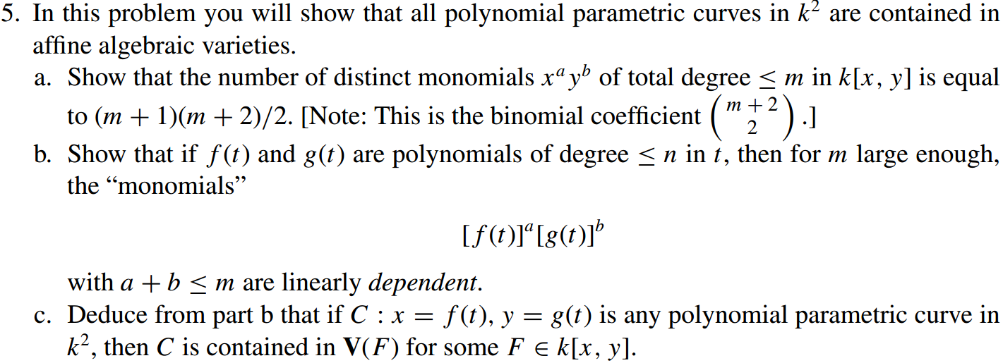
For part (a), the number of monomials is easy to count by listing them in a pyramid like this

$
\begin{array}{cccc}
   x^0 &            &        &        \\
   x^1 & y^1        &        &        \\
   x^2 & x^1y^1     & y^2    &        \\
\cdots & \cdots     & \cdots &  \\
   x^m & x^{m-1}y^1 & \cdots & y^m
\end{array}
$

Now counting them is trivial, it is just $ 1 + 2 + \cdots + (m + 1) = \frac{(m+1)(m+2)}{2} $

For part (b), I read part (c) as a hint. It doesn't quite mention what does it mean by "monomial" and "linear dependent".

I figured it actually means regarding polynomial as vectors. Notice when we add two polynomials, we need to match the degree when we add terms together, so a polynomial is really a vector (can be think of as tuple of numbers).

Now, let imagine if we expand $ [f(t)]^a[g(t)]^b $, the lowest degree term is constant, and the highest degree term is $ t^{na}t^{nb} \le t^{mn} $, and the expansion could have terms of any power of $ t $ in between. We can then think of them as vector space of dimension $ mn + 1 $

If we think of the collection of all polynomials of form $ [f(t)]^a[g(t)]^b $, by part (a), there are $ \frac{(m+1)(m + 2)}{2} $ of them, and all of them are vectors of dimension $ mn + 1 $, so if $ \frac{(m+1)(m + 2)}{2} > mn + 1 $, then by definition these vectors must be linear dependent.

As for part (c), we know those 'vectors' are linear dependent. We can find ourselves a formula $ \sum a_i p_i = 0 $, because these $ p_i $ are just $ x^a y^b $, so the overall formula is a polynomial in $ k[x, y] $.

Suppose a point is on the parametric curve, we know for sure that it is on the polynomial we found. On the other hand, for a point on the polynomial, we do NOT really know if it is on the parametric curve or not, that's why the problem is carefully crafted and say that the parametric curve is contained in the variety, not that the parametric curve IS the variety.

Part (d) is basically the same idea as part (b) and (c) except we go up one dimension. We consider the 'monomial' $ [f(t, u)]^a[g(t, u)]^b[h(t, u)]^c $.

To count the number of these 'monomials', we need to be more imaginative. Consider a pile of balls arranged in a tetrahedral shape like this.

The red ball represents the 'monomial' $ [f(t,u)]^0[g(t, u)]^0[h(t, u)]^0 $, the blue ball represents $ [f(t,u)]^1[g(t, u)]^0[h(t, u)]^0 $ and so on. The total number of 'monomials' is known as the tetrahedral numbers and there is $ \frac{m(m+1)(m+2)}{6} $ of them.

The total number of terms in such expression, however, is going to be bounded by the degree of $ t $ and $ u $ just like what we did in part (b). The maximum degree in $ t $ and $ u $ is both mn. So there can be at most $ (mn + 1)^2 $ terms.

Therefore we can still pick $ m $ such that $ \frac{m(m+1)(m+2)}{6} > (mn+1)^2 $ and therefore we can still argue for the vectors being linearly dependent.

Once we have that linear dependency, we can have the  $ \sum a_i p_i = 0 $ expression again, and once again that will be our $ F $ for the surface case!

UTM Ideals Varieties and Algorithm - Chapter 2 Section 1 Exercise 4

Problem:

Solution:

For part (a), in order to show a set is an ideal, we check the two conditions for ideals.

Condition 1: If $ a \in I $, then $ h a \in I $ for all $ h \in R $.

This is true for I because if $ a \in I $, then $ a = x_{t_1}f_1 +  \cdots + x_{t_m}f_m $,
so $ ha = h(x_{t_1}f_1 +  \cdots + x_{t_m}f_m) = x_{t_1}(hf_1) +  \cdots + x_{t_m}(hf_m) \in I $.

Condition 2: If $ a \in I $ and $ b \in I $, then $ a + b \in I $.

This is also true because

$ a \in I $, then $ a = x_{t_1}f_1 +  \cdots + x_{t_m}f_m $,
$ b \in I $, then $ b = x_{u_1}g_1 +  \cdots + x_{u_m}g_m $,

The sum then must also be the same form and therefore $ a + b \in I $.

For part (b), if $ I $ has a finite generating set, then each element is a polynomial and therefore by definition above, a finite linear combination of monomials.

Therefore the number of variables involved in that finite generating set must be finite, but the ideal has infinite number of variables. So there cannot be a finite generating set.

UTM Ideals Varieties and Algorithm - Chapter 2 Section 1 Exercise 3

Problem:

Solution:

For part (a), note that according to the errata, the last equation should be $ x_3 = -t + 6 $.

First note that all the equations are linear and there is one parameter, it is a line. We should expect two linear equations defining two planes.

From the first equation, it is obvious that $ t = x_1 + 5 $, so we get from the second equation $ x_2 = 2t + 1 = 2 (x_1 + 5) + 1 = 2x_1 + 11 $, and from the third equation $ x_3 = -t + 6 = -(x_1 + 5) + 6 = 1 - x_1 $, so the solution is:

$ x_2 = 2x_1 + 11 $
$ x_3 = 1 - x_1 $

Part (b) is more complicated, it is a two dimensional 'plane' in a 4 dimensional space. Adhoc methods like the previous problem does not work great, so we will try something different. We model the problem using this matrix.

$ \begin{array}{ccccccc}t & u & x_1 & x_2 & x_3 & x_4 & t\\2 & -5 & -1 & 0 & 0 & 0 & 0\\1 & 2 & 0 & -1 & 0 & 0 & 0\\-1 & 1 & 0 & 0 & -1 & 0 & 0\\1 & 3 & 0 & 0 & 0 & -1 & 0\end{array} $

Next, we find the reduced row echelon form using MATLAB (using the function rref), and we get this.

$ \begin{array}{ccccccc}t & u & x_1 & x_2 & x_3 & x_4 & t\\1 & 0 & 0 & 0 & 0.75 & -0.25 & 0\\0 & 1 & 0 & 0 & -0.25 & -0.25 & 0\\0 & 0 & 1 & 0 & 2.75 & 0.75 & 0\\0 & 0 & 0 & 1 & 0.25 & -0.75 & 0\end{array} $

We claim that the last two rows is our solution. To see that, any point that satisfied the parametrization must satisfy all four equations, and therefore it satisfy the last two. For any point satisfy the last two equations, we can always find $ t $ and $ u $ by equation 1 and 2, so we have proved the answer is

$ x_1 + 2.75x_3 + 0.75x_4 = 0 $

$ x_2 + 0.25x_3 - 0.75x_4 = 0 $

Part (c) is pretty easy, it is simple to inspect the answer is

$ x^4 = y $

$ x^7 = z $

Differential Geometry of Curves and Surfaces - Chapter 1 Section 3 Exercise 2

Problem:

Solution:

We will skip part (a) because it is basically the same as this previous exercise. The solution is $ (t - \sin t, 1 - \cos t) $

For part (b), we compute the arc length as

$ \begin{eqnarray*} & & \int\limits_{0}^{2\pi}{\left|\alpha'(t)\right|dt} \\ &=& \int\limits_{0}^{2\pi}{\sqrt{\alpha'(t) \cdot \alpha'(t)}dt} \\ &=& \int\limits_{0}^{2\pi}{\sqrt{(1-\cos t)^2 + \sin^2 t}dt} \\ &=& \int\limits_{0}^{2\pi}{\sqrt{1 - 2\cos t + \cos^2 t + \sin^2 t}dt} \\ &=& \int\limits_{0}^{2\pi}{\sqrt{2 - 2\cos t}dt} \\ \end{eqnarray*} $

The rest is really just an integration problem, let $ x = \cos t $, so

$ \begin{eqnarray*} dx &=& -\sin t dt \\ &=& -\sqrt{1 - \cos^2 t} dt \\ &=& -\sqrt{1 - x^2}dt \\ dt &=& \frac{dx}{-\sqrt{1-x^2}} \end{eqnarray*} $

When $ t = 0 $, $ x = \cos 0 = 1 $
When $ t = \pi $, $ x = \cos \pi = 0 $

$ \begin{eqnarray*} & & \int\limits_{0}^{2\pi}{\sqrt{2 - 2\cos t}dt} \\ &=& 2\int\limits_{0}^{\pi}{\sqrt{2 - 2\cos t}dt} \\ &=& 2\int\limits_{1}^{-1}{\sqrt{2 - 2x}\frac{dx}{-\sqrt{1-x^2}}} \\ &=& 2\int\limits_{-1}^{1}{\sqrt{\frac{2 - 2x}{1-x^2}}dx} \\ &=& 2\sqrt{2}\int\limits_{-1}^{1}{\sqrt{\frac{1}{1 + x}}dx} \\ &=& 4\sqrt{2}\sqrt{1+x}|_{-1}^{1} \\ &=& 8 \\ \end{eqnarray*} $

Just as an aside, I used numerical integration and arc length approximation to make sure the answer is correct.

Differential Geometry of Curves and Surfaces - Chapter 1 Section 3 Exercise 1

Problem:

Solution:

The tangent line has direction $ \vec{a} = (3, 4t, 8t^2) $
The given line has parametric form $ (u, 0, u) $ so it's direction $ \vec{b} (1, 0, 1) $

The angle between these two direction is $ \frac{\vec{a} \cdot \vec{b}}{|\vec{a}||\vec{b}|} = \frac{(3 + 8t^2)}{\sqrt{3^2 + (4t)^2 + (8t^2)^2}\sqrt{1^2 + 0^2 + 1^2}} = \frac{(3 + 8t^2)}{\sqrt{9 + 16t^2 + 64t^4}\sqrt{2}} = \frac{(3 + 8t^2)}{\sqrt{(3 + 8t^2)^2}\sqrt{2}} = \frac{1}{\sqrt{2}}$

So the angle is constant.

Differential Geometry of Curves and Surfaces - Chapter 1 Section 2 Exercise 5

Problem:

Solution:

$ |\alpha(t)| $ is a constant if and only if $ \alpha(t) \cdot \alpha(t) $ is a constant, so we focus on the latter, as a differentiable function of $ t $. Now it is differentiable and it is constant, then its derivative must be 0.

$ (\alpha(t) \cdot \alpha(t))' = 2 \alpha(t) \cdot \alpha'(t) $ so we know $ |\alpha(t)| $ is a constant if and only if the two vectors $ \alpha(t) $ and $ \alpha'(t) $ are orthogonal.

Differential Geometry of Curves and Surfaces - Chapter 1 Section 2 Exercise 4

Problem:

Solution:

Consider the function $ \alpha(t) \cdot v $, it is a differentiable function of $ t $, now $ (\alpha(t) \cdot v)' = 2\alpha'(t) \cdot v = 0 $ as the vectors are orthogonal. So $ \alpha(t) \cdot v $ is a constant function, and therefore $ \alpha(t) $ is orthogonal to $ v $ for all $ t $.

Differential Geometry of Curves and Surfaces - Chapter 1 Section 2 Exercise 3

Problem:

Solution:

Note that $ \alpha''(t) = 0 \implies \alpha'(t) = (a, b, c) $ is constant independent of t, so $ \alpha(t) = (at + x_0, bt + y_0, ct + z_0) $ is a straight line.

Differential Geometry of Curves and Surfaces - Chapter 1 Section 2 Exercise 2

Problem:

Solution:

The squared distance between $ \alpha(t) $ and the origin is $ \alpha(t) \cdot \alpha(t) $. It is a differentiable function of $ t $ and it reaches minimum at $ t_0 $, so $ (\alpha(t_0) \cdot \alpha(t_0))' = 0 $

Using the product rule, we get $ \alpha'(t_0) \cdot \alpha(t_0) = 0 $, now both vectors are non zero so they must be orthogonal.

Differential Geometry of Curves and Surfaces - Chapter 1 Section 2 Exercise 1

Problem:

Solution:

$ \alpha(t) = (\cos t, -\sin t) $.

Be careful with the clockwise direction.

Differential Geometry and Its Application - Exercise 3.1.10

Problem:

Solution:

A surface is minimal if its mean curvature is 0, so the sum of the eigenvalues is 0. Let the eigenvalues be $ x $ and $ y $ respectively, the Gaussian curvature K is then the product $ xy = x(-x) = -x^2 \le 0 $

Differential Geometry and Its Application - Exercise 3.1.9

Problem:

Solution:

Let's compute the shape operator for the cylinder. First, we parametrize the cylinder as follow:

$ (R \cos u, R \sin u, v) $.

$ x_u = (-R \sin u, R \cos u, 0) $.
$ x_v = (0, 0, 1) $.

The normal vector is $ x_u \times x_v = (R \cos u, R \sin u, 0) $

The unit normal vector is then $ (\cos u, \sin u, 0) $

$ S_{p}(x_u) = -\nabla_{x_u}U = (x_u[\cos u], x_u[\sin u], x_u[0]) = (\frac{\partial \cos u}{\partial u}, \frac{\partial \sin u}{\partial u}, \frac{\partial 0 u}{\partial u}) = (-\sin u, \cos u, 0) $

$ S_{p}(x_v) = -\nabla_{x_v}U = (x_v[\cos u], x_v[\sin u], x_v[0]) = (\frac{\partial \cos u}{\partial v}, \frac{\partial \sin u}{\partial v}, \frac{\partial 0 v}{\partial v}) = (0, 0, 0) $

Now, if we write a vector on the tangent plane using $ x_u $ and $ x_v $ as basis, then we know the shape operator can be written as a matrix $ \left(\begin{array}{cc}A & B\\C & D\end{array}\right) $

$ S_{p}(x_u) = \frac{1}{R}x_u \implies \left(\begin{array}{cc}A & B\\C & D\end{array}\right)\left(\begin{array}{c}1 \\ 0\end{array}\right) = \left(\begin{array}{c}\frac{1}{R} \\ 0\end{array}\right) $

$ S_{p}(x_v) = 0 \implies \left(\begin{array}{cc}A & B\\C & D\end{array}\right)\left(\begin{array}{c}0 \\ 1\end{array}\right) = \left(\begin{array}{c}0 \\ 0\end{array}\right) $

So the overall shape operator matrix is simply $ \left(\begin{array}{cc}\frac{1}{R} & 0\\0 & 0\end{array}\right) $, and therefore its eigenvalues are $ \frac{1}{R} $ and $ 0 $, so the mean curvature is $ \frac{1}{2R} $ and the Gaussian curvature is $ 0 $.

That is why the surface is flat, but not minimal.

UTM Ideals Varieties and Algorithm - Chapter 2 Section 1 Exercise 2

Problem:

Solution:

For part (a), we can use MATLAB to compute the reduced row echelon form quickly.

rref([[2 3 -1;1 -1 0;3 7 -2] [9;1;17]])

That gives

   1.00000   0.00000  -0.20000   2.40000
   0.00000   1.00000  -0.20000   1.40000
   0.00000   0.00000   0.00000   0.00000

which means

$ x - 0.2z = 2.4 $
$ y - 0.2z = 1.4 $

That give the parametrization $ (2.4 + 0.2t, 1.4 + 0.2t, t) $

For part (b), we could use MATLAB again, but it is simple so I will skip and do that manually.

It is obvious that we need two parameters, and it is easy to have $ x_1 = u $ and $ x_3 = v $ as the parameters, so the second equation gives $ x_2 = u + v $.

The first equation then give $ u + (u + v) - v - x_4 = 0 $, so the parametrization is $ (u, u + v, v, 2u) $.

For part (c), the answer is right in front of us if we simply let $ x = w $ be the parameter, so the parametrization is simply $ (w, w^3, w^5) $.

UTM Ideals Varieties and Algorithm - Chapter 2 Section 1 Exercise 1

Problem:

Solution:

What would you do if you already have a hammer and you are seeing a nail?

Nail it!

My program for computing GCD and division just fit the purpose, so i just do it.

from polynomial_module import *

# check if polynomial poly is in the ideal defined by the collection of polynomials in ideal
def is_in_ideal(poly, ideal):
    gcd = ideal[0]
    i = 1
    while (i < len(ideal)):
        gcd = polynomial.polynomial_gcd(gcd, ideal[i])
        i = i + 1
    (quotient, remainder) = polynomial.polynomial_divide(poly, gcd)
    return remainder.isZero()
    
def problem_2_1_1():
    print is_in_ideal(polynomial.from_string("x^2 - 3x + 2"), [polynomial.from_string("x - 2")])
    print is_in_ideal(polynomial.from_string("x^5 - 4x + 1"), [polynomial.from_string("x^3 - x^2 + x")])
    print is_in_ideal(polynomial.from_string("x^2 - 4x + 4"), [polynomial.from_string("x^4 - 4x^2 + 12x - 8"), polynomial.from_string("2x^3 - 10x^2 + 16x - 8")])
    print is_in_ideal(polynomial.from_string("x^3 - 1"), [polynomial.from_string("x^9 - 1"), polynomial.from_string("x^5 + x^3 - x^2 - 1")])

The answers are:

a) Yes
b) No
c) Yes
d) Yes

Integrating unit step and delta

In the previous problem, I was working on some piecewise linear functions and doing calculus there. Having many cases is just error prone. Now I try to do thing more algebraically.

The first thing I notice is integrating delta function is simply sampling property, but it applies only if the integrating domain contains 0, that make three cases and it is just not pleasant.

Now, let 'simplify' using step functions.

$ \int\limits_{a}^{b}{\delta(x)f(x)dx} = (\theta(b) - \theta(a))f(x) $

Similarly, we also have this:

$ \int\limits_{a}^{b}{\theta(x)f(x)} = \theta(b)(F(b) - F(0)) - \theta(a)(F(a) - F(0)) $.

To check these, one just consider all 6 permutations of $ a $, $ b $ and $ 0 $. 

Duck Pond Chance (4)

Last post we computed the CDFs for b condition on A, let's compute the PDFs now.

To efficiently compute the derivatives, it is much easier if we have good notations instead of messing with all the cases, so Heaviside step function.

$ P(b \le t|a) = \theta(t - 2a)\frac{t - a}{\pi} $. for $ a \le \frac{\pi}{3} $

By the product rule, we can differentiate and get this, where $ \delta $ is the Dirac delta function.

$ p(b|a) = \delta(t - 2a)\frac{t - a}{\pi} + \theta(t - 2a)\frac{1}{\pi} $.

$ p(a) = \frac{2}{\pi} $, so we integrate to get $ p(b) = \int\limits_{0}^{\frac{\pi}{2}}{p(a)p(b|a)da} $.

Since the function change at $ t - 2a $, let $ y = t - 2a $

$ \frac{dy}{-2} = da $
When $ a = 0 $, $ y = t $.
When $ a = \frac{\pi}{2} $, $ y = t -2\pi $.

$ \begin{eqnarray*} & & p(b) \\ &=& \int\limits_{0}^{\frac{\pi}{2}}{p(a)p(b|a)da} \\ &=& \int\limits_{0}^{\frac{\pi}{2}}{\frac{2}{\pi} (\delta(t - 2a)\frac{t - a}{\pi} + \theta(t - 2a)\frac{1}{\pi}) da} \\ &=& \int\limits_{t}^{t - \pi}{\frac{2}{\pi} (\delta(y)\frac{t + y}{2\pi} + \theta(y)\frac{1}{\pi}) \frac{dy}{-2}} \\ &=& \int\limits_{t - \pi}^{t}{\frac{1}{\pi} (\delta(y)\frac{t + y}{2\pi} + \theta(y)\frac{1}{\pi}) dy} \\ \end{eqnarray*} $

The first term is easy, using the sampling property of the delta function, the integral is simply $ \frac{t}{2\pi^2} $ if $ t \in [0, \pi] $, or 0 otherwise.
The second term is slightly more complicated, it is 0 if $ t < 0 $, $ \frac{t}{\pi^2} $ if $ t \in [0, \pi] $ and $ \frac{1}{\pi} $ if $ t > \pi $.
Although the integration seems to show $ p(b) = \frac{1}{\pi} $ for all $ t > \pi $, but in fact the maximum value of $ t $ is simply $ \frac{4\pi}{3} $, as we already know it caps there. As a sanity check, the area under curve is 1, and the area under curve for $ t \in [0, \pi] = \frac{3}{4} $, which is correct.

EDIT: There are at least two problems I spotted. First, the CDF should also include a term to cancel out the linear growth when it reaches $ a + \pi $. Second, the CDF only applies up to $ a \le \frac{\pi}{3} $.

Duck Pond Chance (3)

Now, let try another approach. We construct the distribution for the smallest enclosing angle incrementally. The case for the smallest enclosing angle for 2 duck is just the uniform distribution in $ [0, \pi] $.

Solving the distribution function for 3 ducks is key, because the same approach is likely useful for 4 ducks, or even $ n $ ducks.

Let $ 2a $ be the smallest enclosing angle for the first 2 ducks
Let $ b $ be the smallest enclosing angle for the first 3 ducks.

For simplicity, we let duck 1 has polar angle $ a $ , duck 2 has polar angle $ -a $.

For duck 3, let it polar angle be $ t $.

If $ t \in [a, -a] $, then $ b = 2a $, in other words, $ P(b = 2a) = \frac{2a}{2\pi} = \frac{a}{\pi} $.

Now suppose $ t \in [a, \pi] $, we need to compare all choices:

(Option 1) duck 2 -> duck 1 -> duck 3 will have angle $ t + a $
(Option 2) duck 1 -> duck 3 -> duck 2 will have angle $ 2\pi - 2a $
(Option 3) duck 3 -> duck 2 -> duck 1 will have angle $ 2\pi - (t - a) = 2\pi + a - t $

We know (option 1) is always as good as than (option 3) because (option 3) - (option 1) = $ (2\pi + a - t) - (t + a) = 2\pi - 2t \ge 0 $ (Remember the maximum of $ t $ is $ \pi $). So we can simply ignore option 3.

It is not so simple for (option 2), we see

(option 1) - (option 2) = $ (t + a) - (2\pi - 2a) = t + 3a  - 2\pi $

We know if the difference is greater than 0, then (option 2) is better. The condition for that to be true is $ t \ge 2\pi - 3a $, which means if the range of $ t = [a, \pi] $ contains $ 2\pi - 3a $, then we need to worry about splitting it so that we choose the options wisely.

For that to happen, $ a \le 2\pi - 3a \implies 4a \le 2\pi \implies a \le \frac{\pi}{2} $, which is automatically true, we also need $ 2\pi - 3a \le \pi \implies \pi \le 3a \implies a \ge \frac{\pi}{3} $

So we have 4 cases to worry about for positive $ t $.

Case 1: $ t \le a $ - in that case $ b = 2a $.
Case 2: $ t \ge a $ and $ a \le \frac{\pi}{3} $ - in that case $ b = t + a $.
Case 3: $ t \ge a $, $ a \ge \frac{\pi}{3} $ and $ t \le 2\pi - 3a $ - in that case $ b = t + a $, and at last
Case 4:  $ t \ge a $, $ a \ge \frac{\pi}{3} $ and $ t > 2\pi - 3a $ - in that case $ b = 2\pi - 2a $.

The cases for negative $ t $ is completely symmetric so we can skip it. Now, if we are given $ a $ and $ t $, we can calculate $ b $.

But, that's not our goal. We wanted to know the distribution of $ b $, To get there, the plan is to compute $ F(b|a) $, the conditional cumulative density function (conditional CDF) for b first.

Case 1 is easy to encode, $ P(b \le t|a) = 0 $ if $ t \in [0, 2a) $.

Case 2 means $ P(b \le t + a|a) = \frac{2t}{2\pi} = \frac{t}{\pi} $, $ a \le \frac{\pi}{3} $ and $ t \ge a $, as the diagram would indicate.

An algebraic manipulation of the above is to let $ s = t + a $, that would give $ P(b \le s) = \frac{s - a}{\pi} $, $ a \le \frac{\pi}{3} $ and $ s \ge 2a $.

Case 1 and Case 2 form the complete distribution for b (condition on a), in this case, we get a curve like this:

Case 3 is getting complicated, as long as we stay within the $ 2\pi - 3a $ region, the probability is pretty much the same as it was for case 2.

$ P(b \le s) = \frac{s - a}{\pi} $, $ a \ge \frac{\pi}{3} $,$ s \ge 2a $ and $ t \le 2\pi - 3a \implies s \le 2\pi - 2a $

Case 4 seems complicated but in fact it is not. It merely says that the $ s $ is capped above by $ 2\pi - 2a $, so the final CDF look like this in that case.

It is too late at night for me now, so I will stop here with the conditional CDF. If time allows I will continue and work on the PDFs.

Duck Pond Chance (2)

Continued with the last post. Here is an implementation of a Monte Carlos simulation.

            Random random = new Random(0);
            const int n = 4;
            int hitCount = 0;
            int labCount = 0;
            for (int i = 0; i < 100000; i++)
            {
                // Represents the angles of the ducks
                double[] d = new double[n];
                for (int j = 0; j < n; j++)
                {
                    // The multiplication by 2 pi is implicit here
                    d[j] = random.NextDouble();
                }
                Array.Sort(d);

                bool hit = false;
                for (int j = 1; j < n; j++)
                {
                    if (d[j] - d[j - 1] > 0.5) // p2 - p1 > pi
                    {
                        hit = true;
                        break;
                    }
                }
                if (!hit)
                {
                    if (d[0] + 1 - d[n - 1] > 0.5) // p1 + 2pi - p4 > pi
                    {
                        hit = true;
                    }
                }

                if (hit)
                {
                    hitCount++;
                }
                labCount++;
            }
            Console.WriteLine((hitCount + 0.0) / labCount);

The code output 0.49947, so we have a good reason to believe the answer is $ \frac{1}{2} $, and that's correct according to the website.

But it is unsettling, this seems too complex and guesswork. There should be a better argument about this.

It is also interesting to note how the probability change as $ n $ changes.

Duck Pond Chance (1)

Problem:

Please find the problem here.

4 small ducks are in a large circular pond, and can each be at any point in the circle with equal chance. What is the probability that a diameter can be drawn so that all 4 ducks are in the same semicircle of the pond?

Solution:

Here is a partial solution to the problem - before we can compute the probability, we need to know a way (i.e. an algorithm) to determine whether or not the ducks are on the same semi-circle.

So this is a computational geometry problem, and we will use computational geometric techniques. Here we will use line sweep (angular sweep).

For simplicity, we simply design a coordinate system such that the pond is the unit circle.

Now, as a probe, let's check if all the ducks are in the upper semi-circle. If all the ducks have positive y coordinate, then we know they are all in the same semi circle, great.

Now, suppose we are not that lucky that some ducks actually have negative coordinate. We will move the diameter to fit them. Now here is the key intuition. Moving it just by a little bit is not going to work, one should move until we reach an 'event point'. If the diameter does not move pass a duck, nothing is going to change.

Therefore the algorithm is to sort the ducks in increasing phase (we model a duck by a complex number in the unit circle) and then we run the line sweep as mentioned above. For simplicity, we always use positive phase (i.e. $ [0, 2\pi) $)

Suppose the line is currently at the first duck with minimal phase $ p_1 $, if the last duck has phase $ p_1 + \pi > p_4 $, then we are good, they are all in the same semicircle.

Suppose that's not true, then we move our sweep line so that it is at the second duck. now we need to make sure the semi-circle contains the 1st duck. The mathematical condition for that to happen is $ p_2 + \pi > p_1 + 2\pi $.

Similarly, we get all these conditions.

$ p_1 + \pi > p_4 $
$ p_2 + \pi > p_1 + 2\pi $
$ p_3 + \pi > p_2 + 2\pi $
$ p_4 + \pi > p_3 + 2\pi $

We can now rearrange these equations into a more illuminating forms:

$ p_1 + 2\pi - p_4 > \pi $
$ p_2 - p_1 > \pi $
$ p_3 - p_2 > \pi $
$ p_4 - p_3 > \pi $

These equations can now be interpreted as the angles between the ducks, if any of these angle is larger than $ \pi $, then we know they fits in a semi-circle. Now can be easily programmed.

Differential Geometry and Its Application - Exercise 2.4.4

Problem:

Solution:

By definition, we have this
$ \nabla_{u_1} U = -S_{p}(u_1) = - k_1 u_1 $

Suppose $ \alpha' = u_1 $, then $ U' = \nabla_{\alpha'} U = \nabla_{u_1} U = -S_{p}(u_1) = - k_1 u_1  =  - k_1 \alpha' $.

Suppose $ \alpha' \ne u_1 $ and $ \alpha' \ne u_2 $ , then $ U' = \nabla_{\alpha'} U = -S_{p}(\alpha') \ne c \alpha' $ for constant $ c $ as $ \alpha' $ is not an eigenvector.

For the second part, as the angle between the surface and the plane is constant, we get

$ U_M \cdot U_P = c $.

So we can take the directional derivative for this one.

$ 0 = \alpha'[U_M \cdot U_P] = \alpha'[U_M] \cdot U_P + \alpha'[U_P] \cdot U_M $

$ -\alpha'[U_M] \cdot U_P = \alpha'[U_P] \cdot U_M $

$ S_p(\alpha') \cdot U_P =0 $

We know $ S_p(\alpha') $ is on the tangent plane. We now also know it is on $ P $, so it has to be $ k\alpha' $. So $ \alpha' $ is an eigenvector of the Weingarten map, and the curve is a line of curvature.

UTM Ideals Varieties and Algorithm - Chapter 1 Section 5 Exercise 17

Problem:

Solution:

This is basically exercising the algorithm we developed in the last problem, the flow goes like this

$ I(V(f_1, f_2)) = I(V(g)) $
$ I(V(g)) = \langle g_{\text{red}} \rangle $
$ g_{\text{red}} = \frac{g}{d} $
$ d = gcd(g, g') $

$ g = x^4 - 2x^3 + 2x - 1 $
$ g' = 4x^3 - 6x^2 + 2 $
$ d = x^2 - 2x + 1 $
$ g_{\text{red}} = x^2 - 1 $

Therefore $ I(V(x^5 - 2x^4 + 2x^2 - x, x^5 - x^4 - 2x^3 + 2x^2 + x - 1)) = \langle x^2 - 1 \rangle $

All these are computed using this program

print "Problem 17"
f = polynomial.from_string("x^5 - 2x^4 + 2x^2 - x")
g = polynomial.from_string("x^5 - x^4 - 2x^3 + 2x^2 + x - 1")
gcd = polynomial.polynomial_gcd(f, g)
gcdd = gcd.derivative()
d = polynomial.polynomial_gcd(gcd, gcdd)
(gred, r) = polynomial.polynomial_divide(gcd, d)
print gcd
print gcdd
print d
print gred

UTM Ideals Varieties and Algorithm - Chapter 1 Section 5 Exercise 16

Problem:

Solution:

The previous exercises basically outlined the whole algorithm.

First, find the GCD, $ g $, of $ f_1, \cdots, f_s $. We know that $ V(f_1, \cdots, f_s) = V(g) $.

Next, compute $ g_{\text{red}} = \frac{g}{GCD(g, g')} $

Now we know $ I(V(f_1, \cdots, f_s)) = I(V(g)) = \langle g_{\text{red}} \rangle $

UTM Ideals Varieties and Algorithm - Chapter 1 Section 5 Exercise 15

Problem:

Solution:

Part (a) is obvious

$ \begin{eqnarray*} & & \frac{f}{GCD(f, f')} \\ &=& \frac{c(x - a_1)^{r_1} \cdots (x - a_n)^{r_n}}{(x - a_1)^{r_1 - 1} \cdots (x - a_n)^{r_n - 1}} \\ &=& c(x - a_1) \cdots (x - a_n) \\ &=& f_{\text{red}} \end{eqnarray*} $

Part (b) is just an application of the formula.

print "Problem 15"
f = polynomial.from_string("x^11 - x^10 + 2x^8 - 4x^7 + 3x^5 - 3x^4 + x^3 + 3x^2 - x - 1")
fd = f.derivative()
g = polynomial.polynomial_gcd(f, fd)
(q, r) = polynomial.polynomial_divide(f, g)
print q

The square free part of the polynomial is $ x^5 + x^2 - x - 1 $

UTM Ideals Varieties and Algorithm - Chapter 1 Section 5 Exercise 14

Problem:

Solution:

Part (a)

$ f' = r(x - a)^{r-1}h + (x-a)^r h' = (x - a)^{r-1}(rh + (x-a) h') $

Therefore $ h_1 = rh + (x-a) h' $, $ h_1(a) = rh(a) + (a - a)h' = rh(a) \ne 0 $.

Part (b)

Using product rule, we differentiate one of the term and keep the rest, and then we sum them up, so the derivative is

$ f' = \sum\limits_{k = 1}^{n}\left(cr(x-a_k)^{r_k - 1}\prod\limits_{j=1, j \ne k}^{n}(x - a_j)^{r_j}\right) $

Therefore, for the final sum, we can always factor out $ (x - a_1)^{r_1 - 1} \cdots (x - a_n)^{r_n - 1}$

$ f' = \prod\limits_{j=1}^{n}(x - a_j)^{r_j - 1} \sum\limits_{k = 1}^{n}\left(cr\prod\limits_{j=1, j \ne k}^{n}(x - a_j)\right) $

Now after factoring out, the $ k $ term is simply $ cr(x - a_1) \cdots (x - a_n) $ (the product goes without $ (x - a_k) $), so the $ k $ term does not vanish for $ a_k $, but all other terms does, That's why $ H $ does not vanish for any $ a_k $.

Part (c)

With part (b), we proved $ (x - a_1)^{r_1 - 1} \cdots (x - a_n)^{r_n - 1} $ is a common factor. The only roots in $ f $ is $ \{ a_1 \cdots a_n \} $, so if the common factor is not greatest, we contradict the fact that $ H $ does not vanish for any of those roots. 

UTM Ideals Varieties and Algorithm - Chapter 1 Section 5 Exercise 13

Problem:

Solution:

Throughout the problem, we let $ f(x) = \sum\limits_{i = 0}^{n} c_i x^i $, $ g(x) = \sum\limits_{i = 0}^{n} d_i x^i $,

Part (a)

$ \begin{eqnarray*} & & (bf)' \\ &=& \sum\limits_{i = 1}^{n} i c_i b x^{i-1} \\ &=& b \sum\limits_{i = 1}^{n} i c_i x^{i-1} \\ &=& bf' \end{eqnarray*} $

Part (b) - suppose the two polynomials do not have same degree, just pad the shorter one with 0 coefficients.

$ \begin{eqnarray*} & & (f + g)' \\ &=& \sum\limits_{i = 1}^{n} i (c_i + d_i) x^{i-1} \\ &=& \sum\limits_{i = 1}^{n} i c_i x^{i-1} + \sum\limits_{i = 1}^{n} i d_i x^{i-1}\\ &=& f' + g' \end{eqnarray*} $

Part (c)

$ \begin{eqnarray*} & & (fg)' \\ &=& ((\sum\limits_{i = 0}^{n}c_i x^i)(\sum\limits_{j = 0}^{n}d_j x^j))' \\ &=& (\sum\limits_{i = 0}^{n}\sum\limits_{j = 0}^{n}c_i d_j x^{i+j})' \\ &=& \sum\limits_{i = 0}^{n}\sum\limits_{j = 0}^{n}(i + j)c_i d_j x^{i+j-1} \\ &=& \sum\limits_{i = 0}^{n}\sum\limits_{j = 0}^{n}ic_i d_j x^{i+j-1} + \sum\limits_{i = 0}^{n}\sum\limits_{j = 0}^{n}jc_i d_j x^{i+j-1} \\ &=& (\sum\limits_{i = 1}^{n}ic_i x^{i-1})(\sum\limits_{j = 0}^{n}d_j x^j) + (\sum\limits_{i = 0}^{n}c_ix^{i})(\sum\limits_{j = 1}^{n}j d_j x^{j-1}) \\ &=& f'g + fg' \end{eqnarray*} $

Note - in the third and fourth equal sign, the double summation should exclude $ i + j = 0 $ case, that would explain the switching of summation limits on the fifth equal sign.

UTM Ideals Varieties and Algorithm - Chapter 1 Section 5 Exercise 12

Problem:

Solution:

Part (a) is simple.

A point is in the variety if it is a root.

For part (b).

$ g \in I(V(f))  \Leftrightarrow g(a_i) = 0 \text{ }, \forall i \Leftrightarrow g = f_{\text{red}}h \Leftrightarrow g \in \langle f_{\text{red}} \rangle $

UTM Ideals Varieties and Algorithm - Chapter 1 Section 5 Exercise 11

Problem:

Solution:

Part (a) is really just another way of stating the fundamental theorem of algebra. Note that the set $ V(f) $ is simply the set of root of $ f $.

Part (b), GCD is 1 $ \Leftrightarrow $ these polynomial do not have a common monic factor $ \Leftrightarrow $ these polynomial does not have a common root $ \Leftrightarrow $ the variety is the empty set.

Part (c), Compute the GCD, and return the variety is empty if the GCD is 1.

UTM Ideals Varieties and Algorithm - Chapter 1 Section 5 Exercise 10

Problem:

Solution:

The key idea is to return more values in each call to GCD.

Function ExtendedGCD(f, g) = (A, B, h):
  if (degree(A) > degree(B)):
    return ExtendedGCD(g, f)
  else:
    (quotient, remainder) = divide(A, B)
    if (remainder == 0):
      # A - B * quotient = 0
      # A + B - B * quotient = B
      # A + B * (1 - quotient) = B
      return (1, 1-quotient, B)
    else
      (p, q, gcd) = GCD(B, remainder)
      # A - B * quotient = remainder
      # p * B + q * remainder = gcd
      # p * B + q * (A - B * quotient) = gcd
      # q * A + (p - q * quotient) * B = gcd
      return (q, p - q * quotient, gcd)

Now even my pseudocode are pythonic!

UTM Ideals Varieties and Algorithm - Chapter 1 Section 5 Exercise 9

Problem:

Solution:

Because the polynomial with a single variable is a principal ideal domain. The ideal $ \langle x^3 + x^2 - 4x - 4, x^3 - x^2 - 4x + 4, x^3 - 2x^2 - x + 2 \rangle $ is essentially generated by their GCD, so we find the GCD of these polynomials using the program we developed for the last problem, it turns out to be $ \langle x - 2 \rangle $.

Now it is obvious that $ x^2 - 4 = (x + 2)(x - 2) \in \langle x - 2 \rangle = \langle x^3 + x^2 - 4x - 4, x^3 - x^2 - 4x + 4, x^3 - 2x^2 - x + 2 \rangle $.

UTM Ideals Varieties and Algorithm - Chapter 1 Section 5 Exercise 8

Problem:

Solution:

The answer for part (a) is $ x^2 + x + 1 $
The answer for part (b) is $ x - 1 $

In order to solve this problem, I could have just use MATLAB/Octave. It seems that the GCD function in Octave does not support symbolic expressions, but I could write a simple script for that in MATLAB.

But instead, in order to practice Python. I wrote the whole symbolic processing and GCD in Python myself. The code for computing the final GCD is very close to what one would do in MATLAB (arguably closer to mathematics, I hate to type 2 * x in MATLAB, 2x is much more mathematically intuitive)

Here is the main function used to solve the problem.

from polynomial_module import *

# Problem 8a
print polynomial.polynomial_gcd(
    polynomial.polynomial_gcd(
        polynomial.from_string("x^4 + x^2 + 1"),
        polynomial.from_string("x^4 - x^2 - 2x - 1")),
    polynomial.from_string("x^3 - 1"))

# Problem 8b
print polynomial.polynomial_gcd(
    polynomial.polynomial_gcd(
        polynomial.from_string("x^3 + 2x^2 - x - 2"),
        polynomial.from_string("x^3 - 2x^2 - x + 2")),
    polynomial.from_string("x^3 - x^2 - 4x + 4"))

Of course, the magic of this problem lies within the polynomial module. I described the module in this post.

Can you solve in a minute?

Problem:

Solution:

Yes I can!

First, note that we only need to find the unit digit, so we can use the binomial theorem to help us to get rid of a lot of noise

$ 264^n \% 10 = (260 + 4)^n \%10 = 4^n \% 10 $.

Next, notice the unit digit pattern in power of 4s.

4
16
64
256

It is just alternating 4 and 6, so the answer unit digit of the first term is 6, and the second term is 4, so the final unit digit is just 0.

By the way, $ 264^{102} + 264^{103} = $

2672061284943160918522454763266223159532013534099073129065764495853122847577901956596137015881471742644503555582762443491090345356529962017230305249153860349231365381334758920717003765678148536467012213716576437712205080690644467304472055027010109440

It takes no time to compute this in python:

>> 264 ** 102 + 264 ** 103

Can you find the green area?

Problem:

Solution:

Fun problem for the morning.

First, our goal is the area on the side:

The equilateral triangle has area is $ \frac{1}{2}a^2 \sin \frac{\pi}{3} = \frac{\sqrt{3}}{4}a^2 $

The sector have area $ \frac{\frac{pi}{6}}{2\pi}\pi a^2 = \frac{1}{12}\pi a^2 $

Therefore the remaining area on the side is $ a^2 - \frac{\sqrt{3}}{4}a^2 - 2(\frac{1}{12}\pi a^2) = a^2(1 - \frac{\sqrt{3}}{4} - \frac{\pi}{6}) $

Next, we want the area of the petal.

The remaining area on the corner is $ a^2 - \frac{1}{4}\pi a^2 = a^2(1 - \frac{\pi}{4}) $

Therefore the petal area is $ a^2(1 - \frac{\pi}{4}) - 2(a^2(1 - \frac{\sqrt{3}}{4} - \frac{\pi}{6})) = a^2(\frac{\sqrt{3}}{2} + \frac{\pi}{12} - 1) $

Finally, the area we wanted is $ a^2 - 2a^2(1 - \frac{\pi}{4}) - 2a^2(\frac{\sqrt{3}}{2} + \frac{\pi}{12} - 1) = a^2(1 - \sqrt{3} + \frac{\pi}{3}) $